The Relationship Between Shooting and Defensive Efficiency
In my last post I took a broad look at how the four factors impact a lineup’s defensive efficiency. This post will take a closer look at the most important factor: shooting.
As a refresher, the data I am using comes from each team’s most used lineup during the ’07-’08 season (view the lineups). I am using a single lineup from each team in an attempt to understand how coaching and the individual players affect defense.
Certainly we would want to use more lineups to try and make inferences about the league as a whole, but that’s not really the goal right now. Ideally, though, the inferences we make about these 5-player unit statistics will be similar to those we make about the entire league.
Breaking Down Shooting
As we learned last time, a lineup’s points per field goal attempt from this data set has a 0.928 correlation with defensive efficiency. No surprise here, but shooting matters more than anything else with respect to defensive efficiency. The point of this study is to examine if there are specific aspects of shooting that matter more than others.
At its most basic level, shooting can be broken down into two areas: 2pt versus 3pt shooting. We can go further, however, and divy 2pt shots up into the low paint (within 6 feet of the basket), the high paint (all other shots in the paint), and mid-range shots (all other 2pt shots). For 3pt shots, we can consider 3pt shots from the corners versus all other 3pt shots.
We could further divide these areas into even smaller regions, but for now I will focus on these 5 general areas: the low paint, high paint, mid-range, corner 3s, and all other 3s.
The 2pt versus 3pt Shot
Before breaking things down further, it’s worth looking at the relationship between 2pt shots, 3pt shots and defensive efficiency. We already know the relationship between overall shot distribution (in terms of points per FGA) and defensive efficiency, but what about the actual shooting percentages from each area?
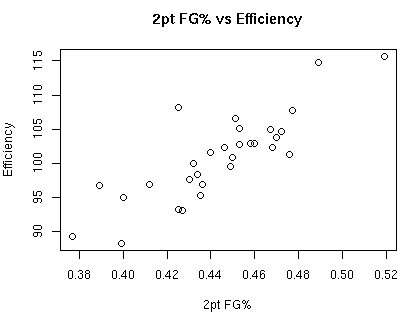
The correlation between 2pt FG% and defensive efficiency is 0.834.
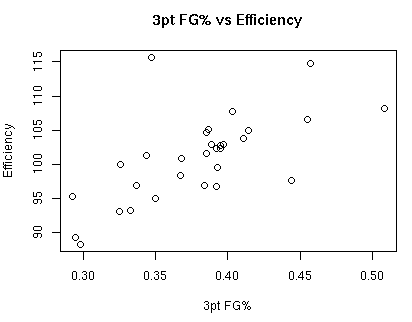
The correlation between 3pt FG% and defensive efficiency is 0.689.
Clearly the distribution of 2pt versus 3pt shots (which has a direct relationship to points per FGA) is most important. That being said, what sort of relationship exists between the distribution of 2pt shots versus 3pt shots and defensive efficiency?
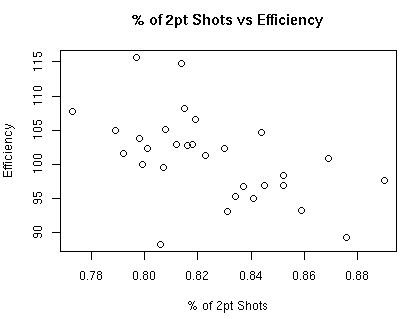
The correlation between the % of shots that are from 2pt range and defensive efficiency is -0.521.
The correlation between the % of shots that are from 3pt range and defensive efficiency is just the inverse relationship to the % of shots that are from 2pt range.
Breaking Down 2pt Shots
As mentioned earlier, I am breaking down 2pt shots into 3 areas: the low paint, the high paint, and mid-range. The low paint is the area in the paint within 6 feet of the basket, the high paint is all other 2pt shots in the paint, and mid-range is all other 2pt shots.
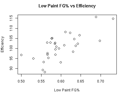
The correlation between low paint FG% and defensive efficiency is 0.707.
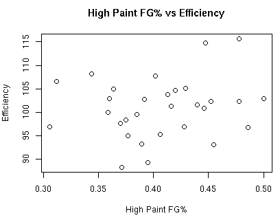
The correlation between high paint FG% and defensive efficiency is 0.177.
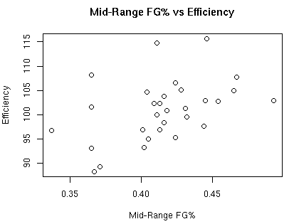
The correlation between mid-range FG% and defensive efficiency is 0.438.
So what about the relationship between the shot distribution of low paint versus high paint versus mid-range shots with respect to overall shot selection? The correlation between % of shots that are in the low paint is 0.155, % of shots that are in the high paint is -0.144, and % of shots that are from mid-range is -0.232.
Breaking Down 3pt Shots
The two areas I will examine for 3pt shots is corner 3pt shots versus all other 3pt shots.
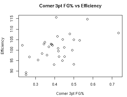
The correlation between corner 3pt shots and defensive efficiency is 0.505.
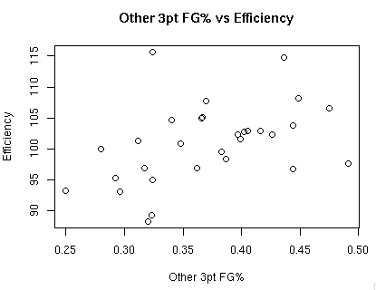
The correlation between all other 3pt shots and defensive efficiency is 0.426.
The correlation for % of shots that are from the corner and defensive efficiency is 0.323, where as the correlation for % of shots that are not from the corner and defensive efficiency is 0.489.
Summary
Talking about correlations isn’t a lot of fun or sexy, but it’s the best way I know of to express the relationship between these shooting statistics and defensive efficiency.
The first point I want to make is that these correlations may not be a good representation for the entire NBA. This analysis is specifically to examine these 30 units and what affects defensive efficiency.
The relative importance of shooting percentages to defensive efficiency is:
- Low Paint FG%: 31%
- Corner 3pt FG%: 22%
- Mid-Range FG%: 19%
- Non-Corner 3pt FG%: 19%
- High Paint FG%: 8%
The relative importance of shot selection to defensive efficiency is:
- Non-Corner 3pt Shots: 36% (decrease shots from here)
- Corner 3pt Shots: 24% (decrease shots from here)
- Mid-Range Shots: 17% (increase shots from here)
- Low Paint Shots: 12% (decrease shots from here)
- High Paint Shots: 11% (increase shots from here)
Lineups that do well in this data set protect the paint and defend the perimeter. This fits well with the conventional wisdom, I’d say, but I’m glad to be able to attach some numbers to the importance of each.
Examining Defense: Defensive Four Factors
Back at the end of September, I made a commitment to get more defensive for this season. To achieve this goal, I’ve been archiving a bunch of NBA games for extracting data to create a better picture of defense.
So to make the best use of my time, I want to ensure I’m getting data that helps create a clearer picture of defense. To do this, I need to know what information would be most helpful to have.
So for the foreseeable future I will be examining various aspects of defense to understand how defensive lineups are built, and what makes a good or bad defensive unit.
The Goal
The real goal in all of this is to get an idea of how coaching and player ability affect overall defensive efficiency and the individual stats that are collected. Because of this, I will be strictly focusing on each team’s most used lineup.
So our main goal is to understand how a new player would fit into a specific lineup and coaching philosophy. We want to know how this player will impact overall defensive efficiency, and how this player will affect various statistics. More data will certainly be helpful, but collecting data for the sake of collecting data isn’t likely to be useful. Hence this process should help focus areas for collecting data.
An Important Assumption
One important assumption in all of this work is the notion that a team’s goal is to minimize their defensive efficiency. A team’s true goal is to maximize their net efficiency (offensive efficiency – defensive efficiency), but we will not be focusing on this for now.
Four Factors
I feel the best place to start examining defense is Dean Oliver’s four factors. These four factors pave the way to examining each component deeper to better understand how defense works.
The Lineups
As I said before, I will be focusing on each team’s most used lineup. By most used, I mean the lineup that was on the court for the most defensive possessions. To make things a little easier, I’ve chosen to estimate possessions instead of count them. I hope this doesn’t prove to be a mistake, but for the interested, I used the “simple” formula for estimating possessions as defined in A Starting Point for Analyzing Basketball Statistics:
Possessions = 0.976 x (FGA + 0.44 x FTA – OREB + TO)
So for each team in the 2007-2008 season, I calculated various statistics for each team and figured out which lineups had the most possessions. These lineups can be found in the 07-08.def.lineups.txt file.
Factor #1: Shooting
Update: My original text is below, but as it turns out Points per FGA = eFG% x 2. Thanks to Ed for pointing this out to me.
Shooting, by no surprise, has been shown to be the most important factor. This factor is often analyzed using effective FG%. I, however, am biased against effective FG%. It is not actually a percentage, and I find it to have no useful mathematical properties (that I’m aware of, at least). Thus I feel compelled to use a shooting statistic that I can make more sense out of.
The statistic I’ve chosen to use is points per field goal attempt. The general idea is that this statistic tells you the expected number of points a defense gives up per shot attempt. The formula is:
Points per FGA = 2 x 2FG% x Pr(2pt Shot) + 3 x 3FG% x Pr(3pt Shot)
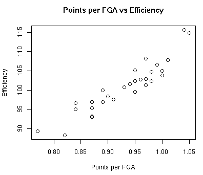
The graph below shows the relationship between points per field goal attempt and defensive efficiency:
The correlation between points per FGA and defensive efficiency is 0.928. So the more points you allow per field goal attempt, the higher your defensive efficiency. Clearly you want to reduce your opponent’s points per FGA.
Factor #2: Turnovers
This factor tells us what percentage of possessions end in a turnover. These turnovers result in a 0 point possession for the opposing offense, so clearly they will have some value.
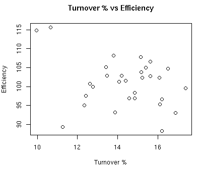
The graph below shows the relationship between turnover % and defensive efficiency:
The correlation between turnover % and defensive efficiency is -0.301. This relationship is much lower than the points per FGA, but an increase in turnover % tends to decrease your defensive efficiency.
Factor #3: Rebounding
This factor tells us what percentage of rebounds the team obtains.
The graph below shows the relationship between rebounding % and defensive efficiency:
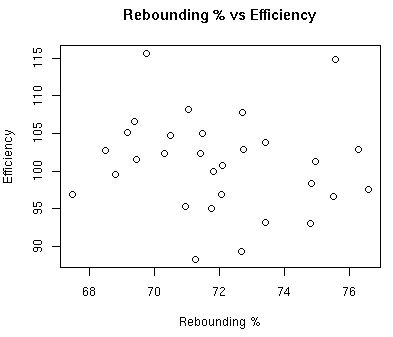
The correlation between rebounding % and defensive efficiency is -0.122.
Factor #4: Free Throws
This factor tells us how many free throws the opponent makes per field goal attempt.
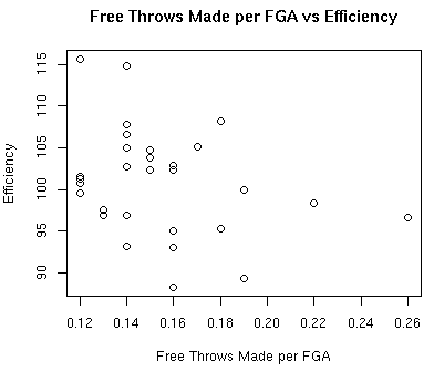
The graph below shows the relationship between free throws made per FGA and defensive efficiency:
The correlation between free throws made per FGA and defensive efficiency is -0.297.
Importance of Each Factor
So one thing we want to know is how important each factor is in terms of defensive efficiency. Ed did some work to show that shooting is worth 45%, turnovers 27%, and rebounding and free throws worth 14% each. The four factor page at B-R.com shows shooting is worth 40%, turnovers 25%, rebounding 20%, and free throws 15%. In Ed’s case, he used team winning % to value the importance of each factor. For B-R.com, I’ve got no idea about the methodology.
The results from this sample show that, with respect to defensive efficiency, shooting is worth 56%, turnovers 18%, rebounding 7%, and free throws 18%. It’s certainly worth gathering a larger sample to truly put some sort of importance weight on each factor, but for this sample it is at least worth looking at.
Summary
There isn’t a lot of ground breaking stuff here that other people haven’t done, but as far as I’m aware of this is the first look at the 5-player unit level.
The next step is to examine each factor in more detail, with the first being shooting. So expect the next post to cover the shooting percentages the lineups allow at various locations on the court.
Daily ’08-’09 Play-by-Play Updates Resumed
Some of the code to update the ’08-’09 play-by-play data broke at the beginning of the year, but I’ve finally gotten around to fixing it.
I know the audience for these daily updates is small, but I just wanted to let those of you that look for the daily updates know that you can now get to them again.
The usual data issues will cause some files not to update automatically, but I’ll fix those soon enough.
Basketball on Paper’s Skill Curves
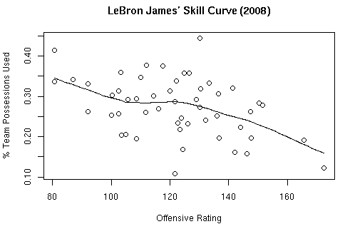
Recent discussion about Basketball on Paper’s skill curves inspired me to use Dean’s formulas to reproduce these curves. The formulas are a bit daunting at first glance, but thankfully they’re really not that bad once you’ve got the data to work with. For the curious reader, most of the formulas came from Appendix 1 of Basketball on Paper.
The Curves
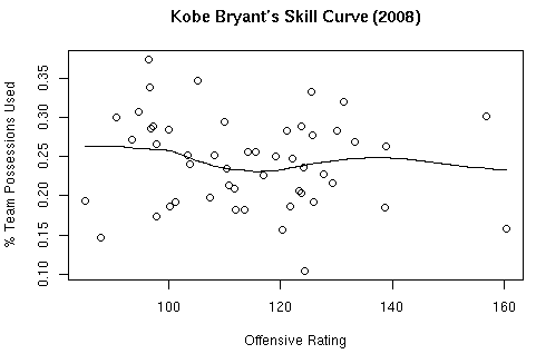
As an initial test of the formulas, I have created skill curves using this season’s data for Kobe Bryant and LeBron James.
Kobe’s Curve:
LeBron’s Curve:
The Code
I used R to perform all of the calculations, so to see how these curves were created, download the skill_curves.zip archive.
Inside of this archive you will find an offense.R file along with some CSV data for Kobe and LeBron. On line 81 of this file is where you can switch between Kobe and LeBron by using the prefix “lebron” or “kobe”.
Summary
I’m pretty sure this is where the data for creating these curves comes from. How Dean actually grouped the data for fitting lines is up for debate. I simply used R’s scatter.smooth function.
Also, please send along any improvements or errors you might find in the code.
UPDATE
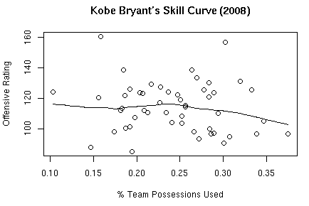
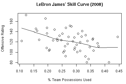
As Neil suggested, here are the images with % Team Possessions Used as the x-axis and Offensive Rating as the y-axis. These definitely make more intuitive sense.
Kobe’s Curve:
LeBron’s Curve:
To replicate these results, change scatter.smooth(ortgs,pused) to scatter.smooth(pused,ortgs) in offense.R.
Predicting Team Rebounding Rates
As we saw in my post on ranking net efficiency ratings, we don’t gain a lot of information by ranking NBA efficiency ratings at the team level. In other words, finding each team’s rating does not affect their overall ranking very much. The same holds true for offensive and defensive rebounding rates, and I suspect it will hold true for the other team statistics that I rate.
That said, these methods give us a framework for understanding the statistics with respect to the entire league. It also allows us to measure the affects of things like home court advantage. This is important, since this information is valuable when making predictions.
So by rating team stats I hope to gain a framework for rating unit stats, which in turn I hope to apply to player stats. Adjusted plus/minus is the current standard for rating players contributions not gathered by traditional statistics, but my goal is to understand how coaching strategy (and other factors) affect these ratings, since the ideal goal is to measure players independent of teammates, opponents, coaching strategy, player usage, etc.
The Method
I have chosen to use a logistic regression to calculate team ratings for offensive and defensive rebounding rates. I chose to use a logistic regression over the Colley Matrix Method because the logistic regression allows me to measure the affect of home court advantage, where as Colley’s method does not allow us to quantify these external factors.
Therefore, to use the ratings listed in the table below you will need to apply the inverse logit function: logit-1(x) = ex / ( 1 + ex )
The Model
Let me first note that this model is with respect to offensive rebounding. So the predicted rates are always in terms of the offensive team.
That said, the intercept for this model is -0.905, and the home court advantage is 0.096.
The team ratings are as follows:
| Team | Offensive Rating | Defensive Rating |
| ATL | -0.117 | -0.008 |
| BOS | 0.016 | -0.249 |
|
CHA |
-0.043 | -0.027 |
| CHI | 0.035 | 0.011 |
| CLE | -0.029 | -0.146 |
|
DAL |
-0.064 | -0.141 |
| DEN | -0.059 | -0.036 |
| DET | -0.091 | -0.141 |
| GSW | -0.052 | 0.165 |
| HOU | -0.089 | -0.185 |
| IND | -0.150 | -0.177 |
| LAC | -0.061 | -0.009 |
| LAL | 0.066 | -0.059 |
| MEM | -0.188 | -0.139 |
| MIA | -0.159 | -0.047 |
| MIL | 0.057 | -0.149 |
| MIN | 0.064 | -0.143 |
| NJN | -0.061 | -0.174 |
| NOH | -0.180 | -0.166 |
| NYK | -0.201 | -0.083 |
| OKC | 0.041 | -0.123 |
| ORL | -0.193 | -0.221 |
| PHI | 0.170 | -0.039 |
| PHX | -0.105 | -0.067 |
| POR | 0.210 | -0.182 |
| SAC | -0.134 | 0.073 |
| SAS | -0.334 | -0.335 |
| TOR | -0.287 | -0.098 |
| UTA | 0.095 | -0.035 |
| WAS | 0 | 0 |
Interpreting These Numbers
In a nutshell, teams with higher the offensive ratings are the best offensive rebounding teams, and teams with lower defensive ratings are the better defensive rebounding teams.
Also, you might be asking yourself the following question: “Why is the Wizard’s offensive and defensive ratings zero?” The answer is because of the way the model is fit. Basically one of the offensive and defensive team’s ratings is “extra information”. In statistical terms, this happens because of singularity.
Since Washington is last alphabetically, they’re the lucky winners of the 0 rating. If the teams were mixed around such that someone else got the 0 ratings, the intercept and ratings for all of the other teams would be different than those listed above. But the interpretations (and predictions) you make would still be the same.
Making Predictions
So the whole point of this is to get an idea of how we might expect one team to rebound against another team. Let’s suppose the Kings are going to Dallas to face the Mavs. The Kings expected offensive rebounding rate would be:
logit-1(-0.905 -0.134 -0.141) = 23.5%
The Mavs expected offensive rebounding rate would be:
logit-1(-0.905 +0.096 -0.064 +0.073) = 31%
In other words, the Mavs and Kings expected defensive rebounding rates would be 76.5% and 69%, respectively.
Summary
Although I did not list the standard errors above, I will say that there is some uncertainty in roughly half the teams ratings. What I mean by that is, their ratings are not statistically signifigant from 0 at traditional levels of signifigance.
Because teams are made up of many 5-player unit combinations and playing situations, there could be many possible explanations for this. So these results have inspired me to fit ratings for last year’s starting 5-player units to see if we can get more confident measures of each 5-player unit’s rebounding rates than we can at the team level.
