Basketball Geek
Advancing our understanding of the game of basketball

A few months ago I took my first look at trying to neutralize rebounding rates. Since that time I’ve given a lot of thought as to what we really want to know about rebounding rates.

In an ideal world we could measure a rating for each player that would allow us to parameterize rebounding rates to determine the percentage of rebounds we would expect each player to obtain under any set of conditions. More importantly than that, we want to know how each player affects his team’s probability of gaining an offensive rebound (even if he doesn’t actually get credit for the rebound).

I certainly don’t live in this ideal world (not yet, at least), so I’m stuck trying to figure out the important things that affect rebounding rates.

The Model

Borrowing from the multilevel model for 3pt shooting, I’ve fit similar models for offensive rebounding rates by grouping players based on position. These models will allow us to estimate some situational effects on player rebounding rates.

The Data

To fit these models I parsed play-by-play data from the 06-07 to 08-09 seasons to determine how many offensive rebounds a player obtained and missed while on the court. I ignored dead ball team rebounds and rebounds off of missed free throws, and I grouped the data by the following categories:

• Game Location: home vs away
• Shot Location: low paint (from <= 6 ft), mid-range (all other 2pt shots), 3pt
• Shooter: did this position shoot the ball?
• Height Difference: number of inches taller (shorter) than the player at the counterpart position

I constrained both lineups such that they consist of a single player at each position. In the event of a “tie”, e.g. two PGs on the court, the players were assigned to the position alphabetically by first name. This is hardly ideal, so it’s something that could certainly be improved in future work. The hope is that this simplicity in choosing positioning doesn’t change our conclusions.

The Fits

Here are the model fits for each position:

PG: logit^-1(-3.57 + 0.04(home) – 0.62(lp) – 0.52(mid) + 0.02(hdiff) – 0.66(shooter) + 2.44(lp*shooter) + 1.2(mid*shooter))

SG: logit^-1(-3.44 + 0.02(home) – 0.5(lp) – 0.39(mid) + 0.03(hdiff) – 0.52(shooter) + 2.72(lp*shooter) + 0.76(mid*shooter))

SF: logit^-1(-3.03 + 0.03(home) – 0.53(lp) – 0.34(mid) + 0.04(hdiff) – 0.89(shooter) + 3.24(lp*shooter) + 0.83(mid*shooter))

PF: logit^-1(-2.57 + 0.05(home) – 0.35(lp) – 0.14(mid) + 0.05(hdiff) – 1.44(shooter) + 3.49(lp*shooter) + 0.78(mid*shooter))

C: logit^-1(-2.45 + 0.05(home) + 0.02(hdiff) – 1.66(shooter) + 3.52(lp*shooter) + 0.71(mid*shooter))

Interpreting The Fits

Based on the predictors listed in the fits above, I have rated each player’s offensive rebounding rate (the so-called random effects) when estimated to be at that position by controlling for home court advantage, shot location, height difference, and “shooter?”.

The only coefficient that isn’t statistically significant at the 0.10 level is the coefficient for (home) in the SG fit. It’s plausible home court advantage doesn’t affect a shooting guard’s probability of gaining an offensive rebound, but the coefficient is reasonably close to the other fits and has the sign we would expect. Thus it seems appropriate to leave it in the model for prediction purposes.

• Home court advantage: We estimate that home court advantage (versus playing on the road) increases the odds of obtaining an offensive rebound by 5% for point guards, 2% for shooting guards, 4% for small forwards, 5% for power forwards, and 6% for centers, controlling for player ability, shot location, height difference, and “shooter?”.
• Not the shooter: We estimate that the odds a point guard obtains the rebound when the shot is taken by another player from the low paint are 0.54 times the odds a point guard obtains the rebound when another player takes a 3pt shot. These estimated odds factors are 0.61 for shooting guards, 0.59 for small forwards, and 0.70 for power forwards. For mid-range shots versus 3pt shots, these estimated odds factors are 0.59, 0.68, 0.71, and 0.87.
• Was the shooter: We estimate that the odds a point guard obtains the rebound when he takes a shot in the low paint are 6.2 times the odds a point guard obtains the rebound when he takes a 3pt shot. These estimated odds factors are 9.2 for shooting guards, 14.9 for small forwards, 22.9 for power forwards, and 33.6 for centers. For mid-range shots versus 3pt shots, these estimated odds factors are 1.97, 1.45, 1.64, 1.91, and 2.04.
• Shooting vs not shooting: We would also like to know what these odds factors are when the player shoots versus does not shoot from these various locations. For shooting from the low paint vs not shooting from the low paint, these estimated odds factors are 5.96 for point guards, 8.96 for shooting guards, 10.44 for small forwards, 7.70 for power forwards, and 6.36 for centers. For shooting from mid-range vs not shooting from mid-range, these estimated factors are 1.72, 1.26, 0.94, 0.52, and 0.34. Shooting from 3pt vs not: 0.52, 0.59, 0.41, 0.24, and 0.19.
• Height Difference: We estimate that each one inch increase in height difference increases the odds of obtaining the rebound by 2% for point guards, 2.9% for shooting guards, 4% for small forwards, 4.6% for power forwards, and 2.4% for centers, controlling for player ability, home court advantage, shot location, and “shooter?”.

Points to Takeaway

Some of these are obvious, but here are the quick points to takeaway from the jumble of odds factors listed above:

• Home court advantage increases our expectation on offensive rebounding rates.
• When not taking the shot, we expect the player to have a lower rebounding rate on shots taken in the low paint and mid-range compared to those taken from 3pt range.
• When taking the shot, we expect the player to have a higher rebounding rate on shots taken in the low paint and mid-range compared to those taken from 3pt range.
• When shooting versus not shooting, we expect a player to have a higher rebounding rate on shots taken in the low paint. We expect higher rebounding rates for guards and lower rebounding rates for all other positions on shots taken from mid-range. We expect lower rebounding rates for all players on 3pt shots.
• Height matters.

Player Ratings for Offensive Rebounding Rates

The following spreadsheet lists the player ratings for offensive rebounding rates:

Player Ratings: Offensive Rebounding Rates

These ratings are in the form of point estimates and confidence intervals for offensive rebounding rates on shots the player does not take. These shots are grouped by location: low paint, mid-range, and 3pt. These estimates are the same at all locations for centers, as we did not measure shot location effects for shots centers did not take.

These point estimates and confidence intervals also took height difference information into account by estimating the mean height of all players listed at each position and subtracting this mean from the height of each player to arrive at our estimated height difference. Although we want to control for players that may be feasting on the undersized, it seems only fair that we give them their height back when making predictions. 😀

Because of the naive way I estimated positioning, you will see players that don’t seem to belong (such as Hassan Adams with point guards). These players aren’t the norm and tend to have a wide range of uncertainty associated with them. So hopefully they are not having a huge impact on the results for the players we care about.

Summary

This model has allowed me to measure the effects of some game situations on offensive rebounding rates, such as shot location and “did the player shoot?”. By using this model we can smooth out the results to give us more realistic estimates than what the 07-08 effective rebounding rates showed.

Major things of interest are controlling for player age, teammate and opponent ability, coaching strategy, and measuring the “other things” that a player may be doing to increase his team’s probability of gaining an offensive rebound. This model assumes none of this matters, so we must think about this sorta stuff when trying to compare player ratings from this model.

The next step I’ll probably take with rebounding is to look at defensive rebounding rates in a similar fashion before trying to come up with a way to model some of the important things mentioned above.

Over the past couple of months I took an awesome class on categorical data analysis. Although it may not sound like it, this sort of data analysis has a lot of application to basketball, as it covers analyzing and building models for things like odds of events, probabilities of success, etc.

Although we didn’t cover it in class, the final chapter in our book by Alan Agresti covered multilevel models (otherwise known as mixed or random effects models). This finally allowed me to start to piece together the large treatment on this topic by Andrew Gelman and Jennifer Hill in their book on regression and multilevel models.

(Hopefully these references provide some reading for those interested in the details of these models.)

An example by Agresti on free throw shooting inspired me to see how we might apply a basic multilevel model to other NBA statistics. I chose 3pt shooting.

The Purpose of a Multilevel Model

The best way for me to explain the purpose of a multilevel model (with respect to sports, at least) is to liken it to a model-based regression to the mean.

By grouping similar players together, we take advantage of what we know about the average player from this group of players with the actual data we collect for each individual player. Like regression to the mean, this allows us to make sense of small samples and intelligently pool the group and individual-specific data together.

Since it’s model based, one advantage of this type of analysis over regression to the mean is that we can more easily quantify effects of the game, like home court advantage, that we might otherwise have a hard time quantifying.

There are more complex multilevel structures that I hope to understand in the future that will hopefully allow for controlling for other aspects of the game. Although not considered here, we might want to control for quality of opponents when rating individual player ability. This is simply one of many things we might want to control for that a more complex model structure may provide over the model presented here.

The Data Used for This Model

The models presented below were fit to a data set containing all 3pt shots attempted from a reasonable distance during the 02-03 through 08-09 seasons. This data set is grouped by the following categories:

• Season
• Player Position: from 1 through 5 to denote PG, SG, SF, PF, and C
• Player Name
• Player Age: as of June 1st prior to the start of the upcoming season
• Home vs Away
• Corner 3pt shots vs Other 3pt shots: a corner 3pt shot is defined to take place within 10ft of the baseline

Here is a sample from the data set that shows Kobe Bryant’s 3pt shots from the 08-09 season:

Season,Position,Name,Age,Game Location,Shot Location,Makes,Misses
2008,2,Kobe Bryant,30,A,corner3,7,7
2008,2,Kobe Bryant,30,A,other3,74,135
2008,2,Kobe Bryant,30,H,corner3,6,14
2008,2,Kobe Bryant,30,H,other3,59,99

Each player’s position is held constant for each season and taken to be the position listed from the most recent season. The position data comes from doug’s stats and the date of birth data comes from database basketball and NBA.com.

The Basic Model Structure

This model considers 3pt shots that are grouped by player. A separate model was fit for each position. The purpose of this model is to estimate each player’s ability while controlling for things like home court advantage, corner 3pt shots vs other 3pt shots, and age effects.

The models below were fit with R using glmer() from the lme4 package.

The Model Fits

PG: logit^-1( -1.40 + 0.02(home) + 0.11(corner3) + 0.053580(age) – 0.000911(age²) )

SG: logit^-1( -0.60 + 0.03(home) + 0.11(corner3) )

SF: logit^-1( -0.64 + 0.04(home) + 0.12(corner3) )

PF: logit^-1( -3.12 + 0.03(home) + 0.10(corner3) + 0.170527(age) – 0.002965(age²) )

The fit for centers does not appear to be that useful. Most centers don’t take that many 3pt shots. It might be better to group centers of interest with power forwards, but for now we’ll ignore these players (sorry Mehmet and Sheed).

All of the coefficients for the fits listed above are significant at the 0.10 level, except for the coefficient for home in the PF fit. It’s about what we would expect it to be at 0.03, so it seems reasonable to leave it in the model.

Interpreting These Fits

First I want to note that failure to converge warnings were encountered when including the age effects in the SG and SF fits, which is the primary reason why we are not controlling for those variables for shooting guards and small forwards. I’ve been unable to resolve this issue, so for now we will assume these players do not have an age effect for their 3pt shots.

That said, here is how we might interpret the effects in these fits:

• Home Court Advantage: We estimate the odds of making a 3pt shot at home are 2% higher than the odds of making a 3pt shot on the road for point guards, controlling for player ability, corner 3pt shots vs other 3pt shots, and age. We estimate this effect to be 3%, 4%, and 3% for shooting guards, small forwards, and power forwards, respectively. From a practical standpoint, we find no evidence that any one position has a higher home court advantage over any other position.
• Corner 3pt Shots: We estimate the odds of making a 3pt shot from the corner are 11.6% higher than the odds of making all other 3pt shots for point guards, controlling for player ability, home court advantage, and age. We estimate this effect to be 11.6%, 12.8%, and 10.5% for shooting guards, small forwards, and power forwards, respectively. Like home court advantage, there is no evidence that any one position has a higher corner3 effect than any other position.
• Aging Curve: We estimate that the peak age for 3pt shooting ability for point guards and power forwards is when these players are 29 years of age.
• Home 3pt FG%: We estimate that the average 29 year old’s non-corner 3pt FG% at home is 35.6% for point guards, 36.1% for shooting guards, 35.4% for small forwards, and 34.6% for power forwards.

The Player Effects

Of ultimate interest here is the player effects that quantify the player ability. Before diving into the numbers, I think it’s worth noting what exactly player ability means in the context of this model. Because we only control for home court advantage, corner 3pt shots vs other 3pt shots, and age, the player ability component is essentially a combination of true player talent, coaching, teammates, opponents, and other things like actual shot selection. A player that suddenly takes nothing but wide open 3pt shots is likely to overperform what we might predict from this model, or underpform if they were able to take the opposite action and only attempt heavily contested 3pt shots. This shot distribution is surely to be affected by coaching, teammates, and opponents.

With that in mind, the following spreadsheet lists 95% confidence intervals for the 3pt shooting ability of each player at home, 29 years of age, and where the uncertainty comes only from the error in the measured ability of each player. The uncertainty associated with the mean intercept, home court advantage, corner3, and age effects are not taken into account.

Spreadsheet: Multilevel Model: Estimated 3pt Ability

Aging Curve Examples

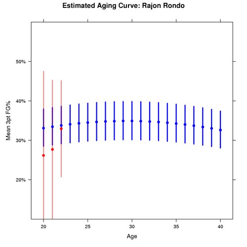
Rajon Rondo has been in the news a lot lately, so I figure he is as good a player as any to take part in showing the estimated aging effect for point guards.

In the graph below the blue represents the predicted mean 3pt FG% for Rajon Rondo weighted based on his actual shot distribution from all seasons in this data set. The red represents the actual estimated mean 3pt FG% for Rajon from those seasons, also weighted based on his actual shot distribution from all seasons in this data set. The dots represent the median, while the lines illustrate the 95% confidence interval for this mean 3pt FG%.

The uncertainty shown is only for the uncertainty in the actual measured player effect. The uncertainty on the age coefficients gives us fairly wide intervals to work with, so this uncertainty has been removed for clarity in the graph. This highlights the lack of precision for the estimated aging curve, even though the coefficients are statistically significant.

For a comparison, here is Steve Nash’s estimated aging curve:

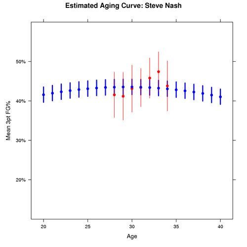
There are two things to take away from this comparison. First, we have more data on Steve Nash, so the uncertainty around his ability is smaller than the uncertainty around Rondo’s ability. This is shown by the smaller bars in Nash’s graph.

Second, the aging effect for point guards is estimated to be fairly small. By that I mean the curve is not very steep, so although the curvature exists, we estimate it to be a fairly flat curve.

Point guards, however, are not the only position we estimated aging effects for. Here are similar graphs comparing a young power forward to a veteran power forward:

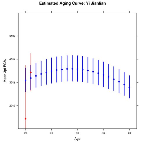
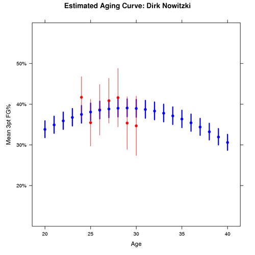
Like Rondo, there is more uncertainty around Jianlian’s ability than Nowitzki’s. Another comparison to the point guards comes in the shape of the curve. As the graphs show, the estimated curve for power forwards is steeper than the estimated curve for point guards.

Recreate These Results

To recreate these results with the R and data files listed below, you will need to install the arm package and its associated dependencies. One easy way to do this should be to run the following command from your R console:

install.packages(“arm”, dependencies=TRUE)

Once you have these packages, you’ll need to download these files:

• multi_3pt.R: By default, this R script simply fits the models above. You can then use summary(fits[[i]]) to see the results, where i = 1, 2, 3, or 4. Edit the code where you see the first if (0) statement to create the graphs above. Edit the code where you see the second if (0) statement to create the CSV file used to generate the spreadsheet above.
• raw_3pt.csv: This CSV data file contains the data as defined in the data section at the beginning of this post.

Summary

This is my first attempt at using a multilevel model with NBA, so there is certainly a mistake or two lying around somewhere. 🙂

I used the simplest structure possible for this model, so my hope is that future research in this area will allow for different groupings. One such grouping would ideally be at the team (or coach?) level.

In my quest to create a realistic simulation of the NBA, I’ve come to the point in which I need to answer an important question: how long does it take for an event to occur after the start of a play?

We don’t actually have to care about the time distribution of events to simulate and make inferences about most player versus player aspects of the game. That said, there are some important aspects of the game that are directly tied to time. By using time, we will be able to better examine how the time-to-penalty situation impacts a team’s efficiency. Although my direct focus as of now is on fouls, other aspects, like strategy, have timing implications, too.

Estimating The Distributions

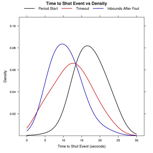
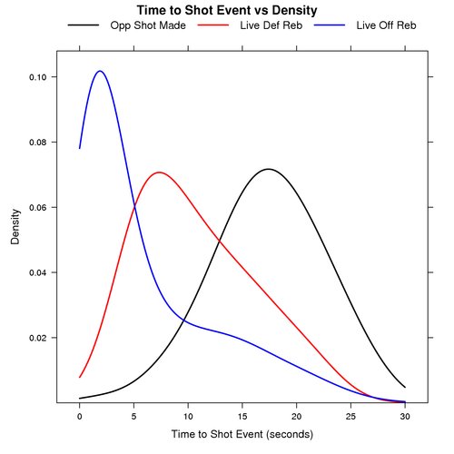
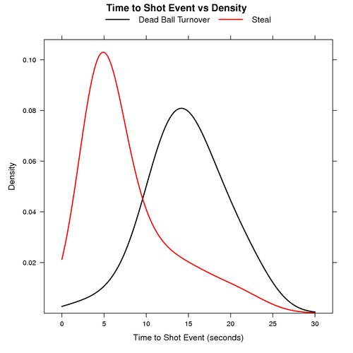
The data used to estimate these time to event distributions was extracted from the 06-07 to 08-09 regular season’s play-by-play data. This data is represented as the number of seconds elapsed from the start of the play to the time of the play ending event, all conditional on how the play started.

Thanks to a tip from @revodavid, I used R‘s density() function to perform kernel density estimation on the data. I’m certainly no expert with this stuff, but for some reason setting adjust to 0.5 (half the default bandwidth) garnered results more to what I was expecting. I don’t want to get too crazy altering the default results, though, as the idea isn’t to follow every little bump in the data, but rather to intelligently smooth the data to provide a good approximation. This isn’t life or death stuff here, so I figure it will be good enough for now.

One thing to point out with the data is that the times aren’t perfectly measured. Time is continuous in nature, yet (prior to the 2009 playoffs, at least) we never see fractional seconds in the play-by-play. The way the data is collected is also inexact. The shot events below show events that last past 24 seconds. Aside from actual errors in the time stamp on each play-by-play event, the shot event time isn’t actually recorded when the shot is taken. Thus we expect to run off more than 24 seconds for some shots.

Time to Shot Events

To illustrate how long events take to occur, I’ve decided to show the estimated probability distributions for the time to shot events. These shot events include all 2pt and 3pt makes, misses, and shooting fouls drawn.

Period Start vs Timeout vs Inbounds After Foul

The graph below shows the probability distribution for the number of seconds that elapse before a shot event for plays that start at the beginning of a period, after a timeout, and inbounds after a foul.

Opponent Shot Made vs Live Def Reb vs Live Off Reb

The graph below shows the probability distribution for the number of seconds that elapse before a shot event for plays that start after an opponent’s made shot, a live defensive rebound, and a live offensive rebound.

Dead Ball Turnover vs Steal

The graph below shows the probability distribution for the number of seconds that elapse before a shot event for plays that start after a dead ball turnover and steals.

Explore These Distributions

The graphs above only illustrate the time to event distributions for shot events. There are other events like personal fouls and turnovers that warrant their own time to event distributions for simulation purposes.

You can use the following files to further examine these and other time to event distributions:

• times.R – This R script creates the graphs above, and has some code that can be used to examine the distributions for personal fouls and turnovers.
• times.csv – This CSV data file contains the elapsed times extracted from the play-by-play from the 06-07 to 08-09 regular seasons.

In the times.csv data file you can see the play starting events and the play ending events that you can then examine with times.R.

Summary

By estimating these distributions, we can now get a general idea as to how much time elapses for various NBA events. This will provide a starting point for being able to realistically simulate actual NBA periods versus simply X number of possessions.

One question worth answering is how useful quick shot or drain the clock strategies are. This opens up a lot of other questions such as: what kind of field goal percentages and turnover rates can we realistically expect using these strategies? Hopefully this is a starting point towards moving in that direction.

My last post took a very general look at how plays end in the NBA. To better understand how the game works, it’s important to know how these distributions vary based on how the play starts.

How Do Plays Start?

Plays can start in a variety of ways. I’ve broken these ways into the following 20 categories (along with tags I have given these events that you will see again).

• The start of the game, quarters, and overtime periods: period_start
• After a timeout: timeout
• After an opponent made shot, after which the ball is brought in out of bounds: 2fg_make, 3fg_make, ft_make
• Defensive rebounds under both dead and live ball situations: dreb_2fg_dead, dreb_2fg_live, dreb_3fg_dead, dreb_3fg_live, dreb_ft_dead, dreb_ft_live
• Offensive rebounds under both dead and live ball situations: oreb_2fg_dead, oreb_2fg_live, oreb_3fg_dead, oreb_3fg_live, oreb_ft_dead, oreb_ft_live
• After a foul that leads to the ball being taken in from out of bounds rather than resulting in free throws: inbounds_after_foul
• Opponent turnovers under both dead and live ball situations: tov_dead, tov_steal

The Distributions

By extracting play-by-play data from the 06-07 to 08-09 seasons, I’ve come up with the following spreadsheet that contains the distributions for each season, separated by home and away:

http://spreadsheets.google.com/ccc?key=rFQ-skpTEnN3P7uyLqtJbGQ

For each season, location, and play starting event, the median and 95% credible interval for the true proportion of each play ending event is listed. These proportions are modeled by a Dirichlet distribution using a noninformative prior distribution.

A Note About Team Offensive Rebounds

While extracting the play-by-play data, I realized that the NBA awards a team offensive rebound when the offensive team misses a shot (and iron) while the 24 second shot clock expires. Thus I’ve made the decision to ignore these shots and only keep the turnovers in these situations.

This is done so that these turnovers don’t skew the distribution of dead ball offensive rebounds, and are instead attributed to the play starting event that led to the original shot. Understanding the time distribution of shots will come later.

Telling the Full Story

Although these distributions are important, they aren’t something we can easily work with visually or by hand. Thus they don’t paint a very good picture as to what is going on just by looking at them.

To solve this, I’ve created some graphs to help paint this picture. These graphs only include some of the more likely play starting events.

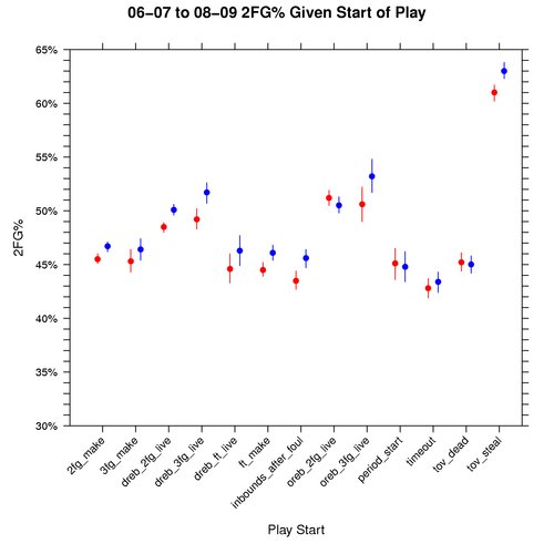
Graph: 2FG% Given Play Start

In order to understand how things like shooting differ between the play starting events, we must condition on knowing that there was a field goal attempt.

The following graph shows this for 2FG% for the 06-07 to 08-09 seasons, where red represents away teams, blue home teams, dots the median, and the lines cover the 95% credible interval:

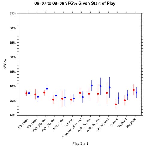
Graph: 3FG% Given Play Start

The following graph shows how 3FG% varies based on the play starting event, conditional on knowing that a 3pt field goal attempt took place. This graph is also for the 06-07 to 08-09 seasons, where red represents away teams, blue home teams, dots the median, and the lines cover the 95% credible interval:

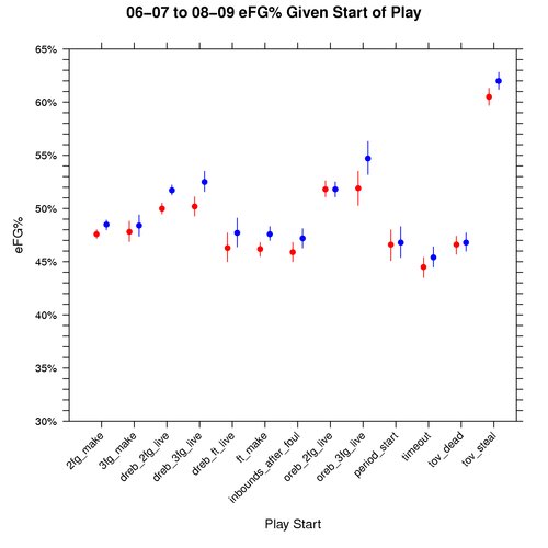
Graph: eFG% Given Play Start

The following graph shows how eFG% (effective FG%) varies based on the play starting event, conditional on knowing that a field goal attempt took place. This graph is also for the 06-07 to 08-09 seasons, where red represents away teams, blue home teams, dots the median, and the lines cover the 95% credible interval:

The 2FG%, 3FG%, and eFG% graphs are drawn to the same scale so that they can be evaluated side by side. One interesting thing about the 2FG% vs eFG% graphs is that all play starting events have a higher eFG% than 2FG% except for tov_steal. This makes me wonder if teams are using the optimal shot distribution for plays that start with a steal.

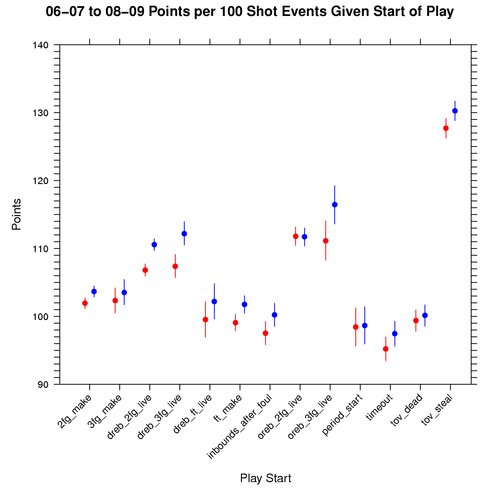
Graph: Points per 100 Shot Events Given Play Start

The following graph shows how many points to expect per 100 shot attempts varies based on the play starting event, conditional on knowing that a shot event took place. This differs from 2FG%, 3FG%, and eFG% in that it illustrates the impact of free throws associated with shooting fouls. Hence a shot event is defined to be all made and missed shots, regardless of whether a shooting foul took place.

To simplify things, I assume the free throws are made at a rate of 75%. In other words, we expect 0.75 points per free throw attempt. This graph is also for the 06-07 to 08-09 seasons, where red represents away teams, blue home teams, dots the median, and the lines cover the 95% credible interval:

Reproduce These Results

There are other ways to work with these distributions than I’ve shown here, so here is how you can reproduce these results and also examine other aspects of the distributions:

• dist.full.csv – This CSV data file contains the distribution of events as counts that are easily fed as parameters to the Dirichlet distribution.
• dist.full.R – Using dist.full.csv, this R script: 1) creates a CSV data file containing the medians and 95% credible intervals for the distributions (as seen in the spreadsheet), and 2) generate the graphs above. It requires the R package MCMCpack for rdirichlet().

Summary

Clearly steals rock when we know a shot took place. There are other events like turnovers (that might lead to a steal) and non-shooting fouls that impact the odds of a team winning any given game. So there is certainly much left to explore.

I’m interested to hear in any results you may find using the data and code listed above.