The Time Distribution of Events in the NBA

In my quest to create a realistic simulation of the NBA, I’ve come to the point in which I need to answer an important question: how long does it take for an event to occur after the start of a play?

We don’t actually have to care about the time distribution of events to simulate and make inferences about most player versus player aspects of the game. That said, there are some important aspects of the game that are directly tied to time. By using time, we will be able to better examine how the time-to-penalty situation impacts a team’s efficiency. Although my direct focus as of now is on fouls, other aspects, like strategy, have timing implications, too.

Estimating The Distributions

The data used to estimate these time to event distributions was extracted from the 06-07 to 08-09 regular season’s play-by-play data. This data is represented as the number of seconds elapsed from the start of the play to the time of the play ending event, all conditional on how the play started.

Thanks to a tip from @revodavid, I used R‘s density() function to perform kernel density estimation on the data. I’m certainly no expert with this stuff, but for some reason setting adjust to 0.5 (half the default bandwidth) garnered results more to what I was expecting. I don’t want to get too crazy altering the default results, though, as the idea isn’t to follow every little bump in the data, but rather to intelligently smooth the data to provide a good approximation. This isn’t life or death stuff here, so I figure it will be good enough for now.

One thing to point out with the data is that the times aren’t perfectly measured. Time is continuous in nature, yet (prior to the 2009 playoffs, at least) we never see fractional seconds in the play-by-play. The way the data is collected is also inexact. The shot events below show events that last past 24 seconds. Aside from actual errors in the time stamp on each play-by-play event, the shot event time isn’t actually recorded when the shot is taken. Thus we expect to run off more than 24 seconds for some shots.

Time to Shot Events

To illustrate how long events take to occur, I’ve decided to show the estimated probability distributions for the time to shot events. These shot events include all 2pt and 3pt makes, misses, and shooting fouls drawn.

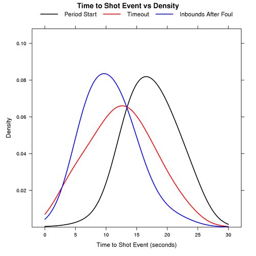
Period Start vs Timeout vs Inbounds After Foul

The graph below shows the probability distribution for the number of seconds that elapse before a shot event for plays that start at the beginning of a period, after a timeout, and inbounds after a foul.

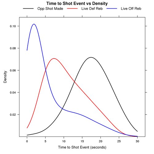
Opponent Shot Made vs Live Def Reb vs Live Off Reb

The graph below shows the probability distribution for the number of seconds that elapse before a shot event for plays that start after an opponent’s made shot, a live defensive rebound, and a live offensive rebound.

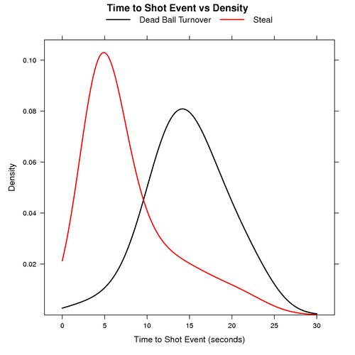
Dead Ball Turnover vs Steal

The graph below shows the probability distribution for the number of seconds that elapse before a shot event for plays that start after a dead ball turnover and steals.

Explore These Distributions

The graphs above only illustrate the time to event distributions for shot events. There are other events like personal fouls and turnovers that warrant their own time to event distributions for simulation purposes.

You can use the following files to further examine these and other time to event distributions:

• times.R – This R script creates the graphs above, and has some code that can be used to examine the distributions for personal fouls and turnovers.
• times.csv – This CSV data file contains the elapsed times extracted from the play-by-play from the 06-07 to 08-09 regular seasons.

In the times.csv data file you can see the play starting events and the play ending events that you can then examine with times.R.

Summary

By estimating these distributions, we can now get a general idea as to how much time elapses for various NBA events. This will provide a starting point for being able to realistically simulate actual NBA periods versus simply X number of possessions.

One question worth answering is how useful quick shot or drain the clock strategies are. This opens up a lot of other questions such as: what kind of field goal percentages and turnover rates can we realistically expect using these strategies? Hopefully this is a starting point towards moving in that direction.