Conditioning the Distribution of Play Ending Events Given How the Play Starts
- 9 Comment
My last post took a very general look at how plays end in the NBA. To better understand how the game works, it’s important to know how these distributions vary based on how the play starts.
How Do Plays Start?
Plays can start in a variety of ways. I’ve broken these ways into the following 20 categories (along with tags I have given these events that you will see again).
- The start of the game, quarters, and overtime periods: period_start
- After a timeout: timeout
- After an opponent made shot, after which the ball is brought in out of bounds: 2fg_make, 3fg_make, ft_make
- Defensive rebounds under both dead and live ball situations: dreb_2fg_dead, dreb_2fg_live, dreb_3fg_dead, dreb_3fg_live, dreb_ft_dead, dreb_ft_live
- Offensive rebounds under both dead and live ball situations: oreb_2fg_dead, oreb_2fg_live, oreb_3fg_dead, oreb_3fg_live, oreb_ft_dead, oreb_ft_live
- After a foul that leads to the ball being taken in from out of bounds rather than resulting in free throws: inbounds_after_foul
- Opponent turnovers under both dead and live ball situations: tov_dead, tov_steal
The Distributions
By extracting play-by-play data from the 06-07 to 08-09 seasons, I’ve come up with the following spreadsheet that contains the distributions for each season, separated by home and away:
http://spreadsheets.google.com/ccc?key=rFQ-skpTEnN3P7uyLqtJbGQ
For each season, location, and play starting event, the median and 95% credible interval for the true proportion of each play ending event is listed. These proportions are modeled by a Dirichlet distribution using a noninformative prior distribution.
A Note About Team Offensive Rebounds
While extracting the play-by-play data, I realized that the NBA awards a team offensive rebound when the offensive team misses a shot (and iron) while the 24 second shot clock expires. Thus I’ve made the decision to ignore these shots and only keep the turnovers in these situations.
This is done so that these turnovers don’t skew the distribution of dead ball offensive rebounds, and are instead attributed to the play starting event that led to the original shot. Understanding the time distribution of shots will come later.
Telling the Full Story
Although these distributions are important, they aren’t something we can easily work with visually or by hand. Thus they don’t paint a very good picture as to what is going on just by looking at them.
To solve this, I’ve created some graphs to help paint this picture. These graphs only include some of the more likely play starting events.
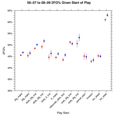
Graph: 2FG% Given Play Start
In order to understand how things like shooting differ between the play starting events, we must condition on knowing that there was a field goal attempt.
The following graph shows this for 2FG% for the 06-07 to 08-09 seasons, where red represents away teams, blue home teams, dots the median, and the lines cover the 95% credible interval:
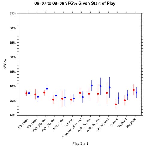
Graph: 3FG% Given Play Start
The following graph shows how 3FG% varies based on the play starting event, conditional on knowing that a 3pt field goal attempt took place. This graph is also for the 06-07 to 08-09 seasons, where red represents away teams, blue home teams, dots the median, and the lines cover the 95% credible interval:
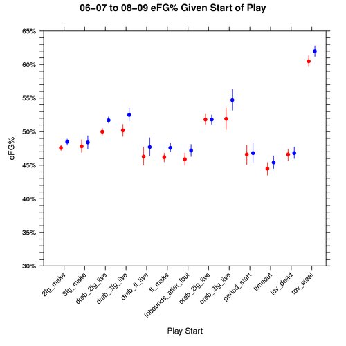
Graph: eFG% Given Play Start
The following graph shows how eFG% (effective FG%) varies based on the play starting event, conditional on knowing that a field goal attempt took place. This graph is also for the 06-07 to 08-09 seasons, where red represents away teams, blue home teams, dots the median, and the lines cover the 95% credible interval:
The 2FG%, 3FG%, and eFG% graphs are drawn to the same scale so that they can be evaluated side by side. One interesting thing about the 2FG% vs eFG% graphs is that all play starting events have a higher eFG% than 2FG% except for tov_steal. This makes me wonder if teams are using the optimal shot distribution for plays that start with a steal.
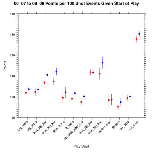
Graph: Points per 100 Shot Events Given Play Start
The following graph shows how many points to expect per 100 shot attempts varies based on the play starting event, conditional on knowing that a shot event took place. This differs from 2FG%, 3FG%, and eFG% in that it illustrates the impact of free throws associated with shooting fouls. Hence a shot event is defined to be all made and missed shots, regardless of whether a shooting foul took place.
To simplify things, I assume the free throws are made at a rate of 75%. In other words, we expect 0.75 points per free throw attempt. This graph is also for the 06-07 to 08-09 seasons, where red represents away teams, blue home teams, dots the median, and the lines cover the 95% credible interval:
Reproduce These Results
There are other ways to work with these distributions than I’ve shown here, so here is how you can reproduce these results and also examine other aspects of the distributions:
- dist.full.csv – This CSV data file contains the distribution of events as counts that are easily fed as parameters to the Dirichlet distribution.
- dist.full.R – Using dist.full.csv, this R script: 1) creates a CSV data file containing the medians and 95% credible intervals for the distributions (as seen in the spreadsheet), and 2) generate the graphs above. It requires the R package MCMCpack for rdirichlet().
Summary
Clearly steals rock when we know a shot took place. There are other events like turnovers (that might lead to a steal) and non-shooting fouls that impact the odds of a team winning any given game. So there is certainly much left to explore.
I’m interested to hear in any results you may find using the data and code listed above.
9 Comments on this post
Trackbacks
-
Trev said:
So you calculate the FG%’s, now what? Some of the results are obvious (higher 2FG% after a steal, i.e. lay-up) but some of the events are not necessarily easy to manufacture. And there is no evidence of causality. How are we to know that the reason that a team shot a higher percentage overall was because they had more “after rebound” events? Some of the analysis has value in scouting: TeamA has a higher 2FG% after DefRebound so we need our guards to get back to increase our defensive posture. But again, there are too many influences into the disparate FG%’s that are not related to the “event” that presumably influence them.
Keep at it man.
June 6th, 2009 at 1:18 pm


[…] Parker is doing some serious freaking work over at his site, the Basketball Geek. Over the weekend, he posted a whole bunch of data measuring the likelihood of a team scoring a […]
[…] + An interesting look at how basketball plays start, and how they end. {Basketball Geek.} […]
[…] are the basic building blocks of basketball, and there is much to explore: how plays end, how a play is likely to end based on how it started, and how long it takes for plays to end are just a starting […]
Conditioning the Distribution of Play Ending Events Given How the Play Starts
https://buddybeds.com/32-dads-who-absolutely-adore-their-dogs/
Conditioning the Distribution of Play Ending Events Given How the Play Starts
https://stmaryskote.in/index.php/2020/01/31/tribal-children-get-together-at-antharasanthe-h-d-kotet/
Conditioning the Distribution of Play Ending Events Given How the Play Starts
https://phamousghana.com/that-guy-good-adekunle-gold-showers-praise-on-king-promise/
Conditioning the Distribution of Play Ending Events Given How the Play Starts
https://saquedemeta.co/doblete-de-uribe-en-mexico/
Conditioning the Distribution of Play Ending Events Given How the Play Starts
http://huntersglenv.com/2021/02/20/homeowners-associations-annual-meeting-of-the-members/