The Distribution of Play Ending Events in the NBA
I have come to the realization that I really don’t understand the NBA game all that well.
Sure I have a general knowledge of basketball, but as I work toward building a realistic simulation of the NBA, I realize that I don’t understand the dynamics of the game that impact a team’s chances of scoring points.
By quantifying the distribution of play ending events, I will be taking the first step in the direction of understanding the dynamics of the game.
What is a play?
The terms possession and play get thrown around a lot, so I want to be clear on the definition of a play that I am using here:
- play – period of play before a play ending event
Ok so that really doesn’t help. The real understanding comes in the definition of a play ending event:
- play ending event – all shot events, any event that stops play or gives the opponent the ball, and any event that creates a free throw opportunity
In general, play ending events can be broken down into four basic categories: fouls, shots, timeouts, and turnovers.
The General Distribution of Play Ending Events
The general distribution of these four basic categories is as follows:
| Season | Location | Foul% | Shot% | Timeout% | Turnover% |
| 08-09 | Away | 8.5% | 75.4% | 5.5% | 10.5% |
| 08-09 | Home | 8.7% | 75.5% | 5.5% | 10.3% |
| 07-08 | Away | 8.3% | 75.6% | 5.4% | 10.6% |
| 07-08 | Home | 8.3% | 76.0% | 5.4% | 10.2% |
| 06-07 | Away | 9.2% | 74.2% | 5.6% | 11.0% |
| 06-07 | Home | 9.2% | 74.1% | 5.8% | 10.9% |
This data was compiled from 137,706, 140,343, and 136,108 away play ending events, and from 136,971, 139,543, and 135,805 home play ending events from the 08-09, 07-08, and 06-07 seasons, respectively.
I believe I need to make it clear that I consider shooting fouls a component of shots, and thus I have grouped them with Shot% and not Foul%. Also, I group offensive foul turnovers with Foul% instead of Turnover%. These distinctions will be made clear below.
One result from this table that interests me is the difference between Foul% and Shot% when comparing the 06-07 season to the other two seasons.
There are enough events to say these are statistically significant from each other, so I’m interested to know if 1) some rule change caused this, 2) some other explanatory reason made this happen that I’m missing (such as the distribution of play starting events, which I will cover in the future), 3) this really was just by chance, or 4) I have some perl code not working as desired.
That said, these general categories give us an idea how plays end, but they don’t really tell us how play ending events for home versus away teams differ. Digging into more detail will shed some light onto this.
Distribution of Fouls
The percentages below are on a per play basis. So this means they are not conditional on knowing there was a foul, which is why they do not sum to 1.
| SEA | LOC | CP | D3S | DP | DT | FT1 | FT2 | OFF | PF | TECH | MISC |
| 08-09 | A | 0.02% | 0.30% | 0.013% | 0.027% | 0.025% | 0.003% | 1.54% | 6.22% | 0.28% | 0.04% |
| 08-09 | H | 0.03% | 0.31% | 0.010% | 0.029% | 0.030% | 0.005% | 1.49% | 6.47% | 0.30% | 0.03% |
| 07-08 | A | 0.02% | 0.32% | 0.011% | 0.026% | 0.027% | 0.001% | 1.55% | 6.09% | 0.25% | 0.02% |
| 07-08 | H | 0.03% | 0.30% | 0.014% | 0.020% | 0.033% | 0.001% | 1.48% | 6.17% | 0.27% | 0.02% |
| 06-07 | A | 0.03% | 0.40% | 0.007% | 0.028% | 0.032% | 0.004% | 1.91% | 6.45% | 0.33% | 0.02% |
| 06-07 | H | 0.03% | 0.39% | 0.005% | 0.020% | 0.035% | 0.003% | 1.77% | 6.65% | 0.31% | 0.03% |
Abbreviations: SEA: Season; LOC: Team Location, A=Away and H=Home; CP: clear path; D3S: defensive 3 seconds (includes all “illegal defense” events for the 06-07 play-by-play); DP: double personal; DT: double technical; FT1: flagrant type 1; FT2: flagrant type 2; OFF: offensive foul; PF: personal fouls; TECH: technicals; MISC: all other fouls.
Distribution of Shots
The percentages below are also on a per play basis.
2 point shots:
| Season | Location | Make% | Miss% | Make+SF% | Miss+SF% | Blocked% |
| 08-09 | Away | 23.4% | 23.3% | 1.93% | 6.96% | 4.26% |
| 08-09 | Home | 24.4% | 23.5% | 1.88% | 6.65% | 3.69% |
| 07-08 | Away | 23.5% | 23.6% | 1.96% | 7.08% | 4.20% |
| 07-08 | Home | 24.7% | 23.7% | 1.81% | 6.83% | 3.58% |
| 06-07 | Away | 25.3% | 28.0% | 2.10% | 7.10% | 4.10% |
| 06-07 | Home | 26.2% | 28.0% | 2.03% | 6.76% | 3.57% |
3 point shots:
| Season | Location | Make% | Miss% | Make+SF% | Miss+SF% | Blocked% |
| 08-09 | Away | 5.60% | 9.73% | 0.025% | 0.113% | 0.109% |
| 08-09 | Home | 5.65% | 9.56% | 0.023% | 0.101% | 0.092% |
| 07-08 | Away | 5.46% | 9.68% | 0.022% | 0.101% | 0.094% |
| 07-08 | Home | 5.55% | 9.65% | 0.029% | 0.105% | 0.087% |
| 06-07 | Away | 2.93% | 4.57% | 0.021% | 0.096% | 0.051% |
| 06-07 | Home | 3.02% | 4.48% | 0.013% | 0.099% | 0.030% |
Distribution of Turnovers
Like the other distributions above, the percentages below are also on a per play basis.
| Season | Location | Steal% | Dead Ball% | ||||
| 08-09 | Away | 6.2% | 4.3% | ||||
| 08-09 | Home | 6.1% | 4.1% | ||||
| 07-08 | Away | 6.2% | 4.4% | ||||
| 07-08 | Home | 6.1% | 4.1% | ||||
| 06-07 | Away | 6.1% | 4.8% | ||||
| 06-07 | Home | 6.1% | 4.7% |
Summary
The distributions presented above are simply one component of plays in the NBA. The next step is to examine how plays start, as this has a role in how a given play ends.
From there, the ultimate goal is to then quantify the distribution of how plays end based on how they started. This will help answer questions like, “What proportion of plays end with a 2pt FG make + shooting foul when the play starts on a steal?” or “Does the data provide evidence that there is a positive or negative relationship with this proportion and playing at home?”
These are simply a couple of examples of the many questions that I want to be able to answer to help better understand how the game works.
Player Statistics at Home vs Away
It has become apparent to me that to we must study the relationship between game situations and the player statistics collected under these game situations before we can fully understand the stats we collect about players. Players enter the game under varying conditions, thus the distribution of game situations is not uniform across all players. Because of this, I feel we can gain insight by studying how these game situations relate to individual player stats.
For example: I’d like to know what sort of relationship garbage time eFG% has to non-garbage time eFG%. This is merely one of many possible questions we can answer by studying game situations.
Home vs Away
The most basic game situation to study is home vs away. We’re all familiar with how much a team’s home court advantage is worth in terms of points or winning percentage, but what about the relationship between a player’s eFG% or turnovers per possession at home vs away?
The Method and Data
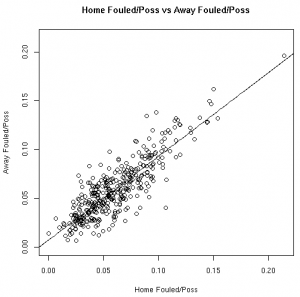
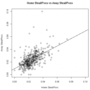
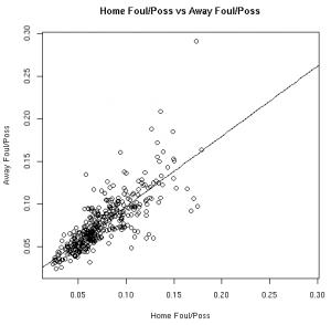
Using data collected for the 2006-2007, 2007-2008, and 2008-2009 regular seasons, I calculated the following statistics for each player: FT%, 2pt FG%, 3pt FG%, eFG%, OReb%, DReb%, turnovers per offensive possession, fouls drawn per offensive possession, personal fouls per defensive possession, and steals per defensive possession.
Using R, I calculated correlation coefficients and fit linear models to the data for all players that took part in at least 100 events at home and away in each category (such as 100 FTA, 100 2FGA, 100 3FGA, 100 offensive possessions, etc). See this file for the raw results.
The Correlation Coefficients
| Year | FT% | 2FG% | 3FG% | eFG% | OR% | DR% | TO% | Fouled% | Steal% | Foul% |
| 06-07 | 0.865 | 0.653 | 0.465 | 0.598 | 0.908 | 0.913 | 0.661 | 0.870 | 0.599 | 0.847 |
| 07-08 | 0.835 | 0.655 | 0.151 | 0.612 | 0.896 | 0.933 | 0.675 | 0.855 | 0.586 | 0.857 |
| 08-09 | 0.816 | 0.614 | 0.346 | 0.540 | 0.905 | 0.899 | 0.670 | 0.856 | 0.561 | 0.798 |
The Relationships in Visual Form
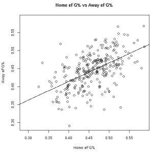
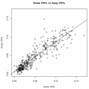
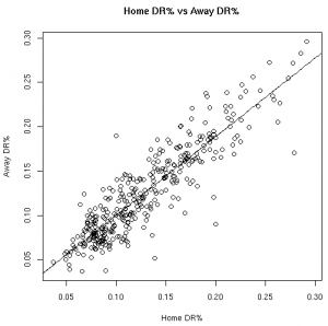
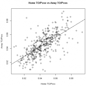
As much fun as it may be to look at correlation coefficients, graphing the data with the fitted linear models helps paint a better picture. The graphs below illustrate these relationships from the 08-09 regular season:
| FT% | 2FG% |
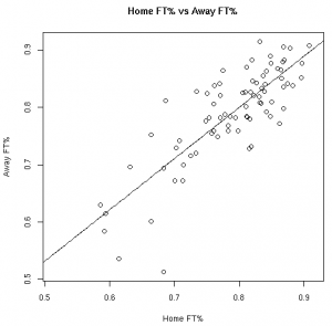 |
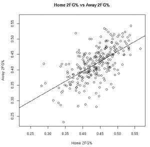 |
| 3FG% | eFG% |
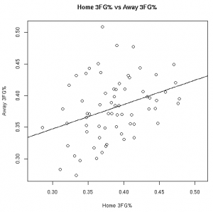 |
 |
| OR% | DR% |
 |
 |
| TO/Poss | Fouled/Poss |
 |
 |
| Steals/Poss | Fouls/Poss |
 |
 |
Making Predictions
The whole point of this is to make some sort of prediction about a player’s stats given some information (such as how they’ve performed at home).
Based on the models fit to this data, knowing a player’s stats at home gives us information about player’s road stats. (Except, of course, for the models fit to the 3FG% data from the 06-07 and 07-08 seasons).
These results, however, should not surprise anyone. Obviously there is a connection between home vs away stats. Hopefully, however, this helps answer the magnitude of the relationship between a player’s stats at home vs away.
My goal is to use the framework outlined above to quantify the relationship between player stats in other game situations of interest (such as garbage time vs non-garbage time).
Reproduce These Results
To reproduce these results, you’ll need to download the following files:
By running source(“home_vs_away.R”) in R, a file with the raw results will be created. Also, to plot the graphs, simply uncomment the plot() code in the home_vs_away() function.
Summary
This data allows us to quantify the relationship between various player stats at home vs away. Other than the before mentioned 3FG% models, all of the linear models showed the home stats to be statistically significant for predicting the away stats. To use these models, see the raw results file.
UPDATE: Per Nick’s suggestion, I’ve re-scaled the graphics so that the x-axis and y-axis cover the same distance.
2006-2007 Regular Season Play-By-Play Data Now Available
I’ve had to focus on other things over the past couple of weeks, so I figured now was as good a time as any to start putting together data sets for past seasons.
’06-’07 Data Set Stats
This regular season data set has 1149 games, which is 81 short of the full season (or 6.6% games short of being complete). As I mentioned with the ’07-’08 data set, I hope to integrate some of these games in the future. That said, this should be a good start.
Downloading the Data
To download the data, visit the data page or use this direct download link.
Why We Need More Data
One key area to study is how things change from season to season, so putting this data together will allow us to do that. With this data, the data from the ’07-’08 season, and data now coming in from the ’08-’09 season, we’ve got 3 years of data to work with.
My current focus will be on putting a few more seasons together so that I’ve got a nice database to work with once the semester is over and some free time on my hands.
Lastly, please let me know if you find any problems with the download. Also, don’t forget about basketballvalue.com if you don’t see a game you’re looking for.
My 2009 NCAA Tournament Odds
Brackets are now closed, and the first NCAA tournament game of the 2009 tournament is about to begin. Therefore, it’s time I post my odds of winning the tournament.
The Method
I used Kenneth Massey’s least squares method to rate and rank each DI team’s net points per possession per game. In other words, I used this method to rate each team’s offensive points per possession – defensive points per possession on a per game basis.
To get a handle on the distribution of the net points per possession, I assumed it to be normally distributed and used the sample standard deviation throughout the season for each team as that team’s standard deviation for this distribution.
With this distribution, I setup the brackets and calculated the odds of each team advancing to each round based on every possible matchup combination in the tournament.
The Odds
The spreadsheet below lists the odds of each team making it to the 2nd round:
http://spreadsheets.google.com/ccc?key=pLJimPjd7oqvl3fE7FW7ZfQ
The spreadsheet below lists the odds of each team making it to the Sweet 16:
http://spreadsheets.google.com/ccc?key=pLJimPjd7oqvc5lqxLiS-Cg
The spreadsheet below lists the odds of each team making it to the Elite 8:
http://spreadsheets.google.com/ccc?key=pLJimPjd7oquqFFKGihAXEw
The spreadsheet below lists the odds of each team making it to the Final Four:
http://spreadsheets.google.com/ccc?key=pLJimPjd7oqt6cOX1w5p2Jg
The spreadsheet below lists the odds of each team making it to the championship game:
http://spreadsheets.google.com/ccc?key=pLJimPjd7oquldaMCLvREeg
The spreadsheet below lists the odds of each team winning the championship:
http://spreadsheets.google.com/ccc?key=pLJimPjd7oqsbYEdXALx7Ew
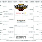
Put all of this together, and you get my bracket:
Who Wins the Title?
These odds suggest UNC is the favorite to win the 2009 championship. That being said, we only expect them to win roughly 9% of the time. Thus we really don’t expect UNC to win the title, as we expect someone else to win it 91% of the time.
Based on a 5 year sample, this method has performed the best. This is clearly a small sample, and weighting the data differently suggests Memphis is the favorite to win (but just at about 11% of the time). This suggests Henry Abbott hasn’t lost his mind. He’s got as good a selection as any.
Thanks
I’d like to thank Dr. Amy Langville, Dr. Martin Jones, Kathryn Pedings, and Patrick Moran for helpful guidance and discussion while fine tuning this method. Also, I’d like to give a shout out to the team from Davidson consisting of Erich Kreutzer and Max Win, who will undoubtedly fall to the competing brackets Kathryn and I submitted to ESPN.
Also, a big thanks to Ken Pomeroy for helping me get points per possession data for the last 5 seasons.
NCAA Teams Do Better When Down at Halftime?
I’ll be the first to admit that I’ve got a long way to go with my education on building and interpreting statistical models, so I find this post by Andrew Gelman very useful.
The post is in response to this article by Jonah Berger and Devin Pope (see discussion here). Here is a quote from Gelman’s post:
I’ll start with their data, which are 6572 NCAA basketball games where the score differential at halftime is within 10 points. Of the subset of these games with one-point gaps at halftime, the team that’s behind won 51.3% of the time. To get a standard error on this, I need to know the number of such games; let me approximate this by 6572/10=657. The s.e. is then .5/sqrt(657)=0.02. So the simple empirical estimate with +/- 1 standard error bounds is [.513 +/- .02], or [.49, .53]. Hardly conclusive evidence!
His full post also provides analysis on one the article’s graphics that he says offers insight into what is going on. Also, Gelman provides commentary on what he would do instead.
Since this post by Gelman is with respect to basketball it is very easy for someone like myself to relate to. Hopefully others out there find this useful as well.
See the full post at Andrew’s blog.
UPDATE
Eli Witus of Count the Basket fame has put together a handy list of discussion on this topic over at the APBRmetrics forum.
