A Basic Hierarchical Model of Efficiency
- 3 Comment
In my last post on retrodicting team efficiency, I set a general baseline that can be used help determine if a new model of team efficiency makes better predictions than a naive model. This is important, as we want to know if added model complexity is worth the hassle.
This post will present a basic hierarchical model of efficiency, and we’ll determine how much better this model is in terms of year to year predictions.
The Model
Like the classical adjusted plus/minus efficiency model, this basic hierarchical model for efficiency is constructed so that we make predictions about the mean number of points scored on a given possession between an offensive and defensive lineup. With this model, though, we consider all player’s offensive and defensive ratings to come from a normal distribution, where we consider two distributions: one for offensive ratings, and one for defensive ratings.
Mathematically, we can write this model as follows:
[latex]Y_{i} \sim {\tt N}(\beta_{0} + \beta_{1} + O_{1} + \cdots + O_{5} + D_{1} + \cdots + D_{5}, \sigma^{2}_{y}) \\ O_{i} \sim {\tt N}(0, \sigma^{2}_{o}) \\ D_{i} \sim {\tt N}(0, \sigma^{2}_{d})[/latex]
Where [latex]\beta_{0}[/latex] estimates the average number of points scored on a possession on the road, [latex]\beta_{1}[/latex] estimates the home court advantage for when the offense is at home, and [latex]O_{i}[/latex] and [latex]D_{i}[/latex] estimate the offensive and defensive ratings for each player, respectively.
Also, because we have to use a Bayesian analysis, all of the parameters and hyperparameters of this model are given non-informative prior distributions.
The Player Ratings
The tables below list this model’s estimated top 10 offensive, defensive, and overall players from the 06-07, 07-08, and 08-09 seasons.
[table id=3 /]
[table id=4 /]
[table id=5 /]
As far as uncertainty in the ratings is concerned, we wouldn’t say that any one of these players is better than the other. Also, there are some cases in which we wouldn’t say that a given player is better than the average player.
Retrodiction Results
Obligatory top 10 lists aside, the real interest is in terms of predictions. Using the retrodiction methodology laid out in the post on retrodicting team efficiency, the ratings from the previous year’s model are used to predict the offensive, defensive, and net efficiency ratings of each team in the next season knowing game location and the 10 players on the court.
The following table lists the results:
[table id=2 /]
The difference in the classical model’s mean absolute error (MAE) and root mean squared error (RMSE) is listed under the MAE Diff and RMSE Diff columns. These are calculated by subtracting the classical model’s result from the hierarchical model’s result. In other words, negative numbers mean our predictions are doing better than the classical model.
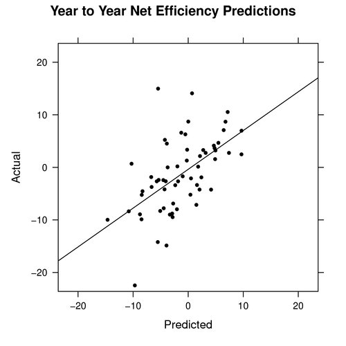
Again, one area of interest is in the net efficiency. The graph below shows the predicted net efficiency versus the actual net efficiency:

Unlike the classical model, this model does not predict teams to have very large or small net efficiency ratings, as most fall within +/- 10 points. This is probably a good thing, since most of the actual ratings fall within this range as well.
Summary
Based on the results above, I consider this basic hierarchical model to better predict efficiency over the classical model.
There is, however, still room for improvement, as we again have some weird results where we predict a net efficiency of -5, yet the actual net efficiency is 15.
Randomness will always give us imperfect results, but this result seems like one that is worth investigating in an effort to provide insight into how we can construct a better model of efficiency.
3 Comments on this post
Trackbacks
-
Kevin Pelton said:
Good stuff, Ryan. Two questions: Does the assumed normal distribution explain why these numbers are smaller than we see with classic adjusted plus-minus?
Second, who’s that outlier at the top of the chart that this method actually predicted to be a below-.500 team?
September 7th, 2009 at 10:02 pm -
Ryan said:
The assumed normal distribution for player ratings keeps us from estimating ratings that are extreme (too big or too small) for players with small sample sizes. So this naturally keeps us from making extreme predictions for the future seasons.
I believe the outlier you’re referring to is the one I mention in the summary. It is the 08-09 Bulls team, where predictions are only made for ~900 possessions since we ignore possessions from guys like D. Rose. I want to better understand why this collection of players did so well, and if we can explain it in any way.
September 7th, 2009 at 10:14 pm -
Ryan said:
I’ve constructed this spreadsheet that lists all offensive and defensive ratings from this model, with associated standard deviations and 95% credible intervals (which are constructed with the 2.5% and 97.5% quantiles).
September 9th, 2009 at 9:55 pm