The Average Number of Starters Over Time
- 1 Comment
For the foreseeable future my work will focus on understanding how specific game situations affect team, unit, and player performance. The end goal is to understand what performance in these specific situations means with respect to true player ability.
To kick this off, I’ve decided to take a very general look at how the average number of starters changes over elapsed game time. First, however, I’ll present the work of another:
Previous Work
Earlier this year, Ben F. over at the APBRmetrics forum created a post called Fun With Charts: Sub Patterns. In this post, Ben linked to a neat tool he created with Open Flash Chart: League Substitution Patterns
This is a pretty cool tool that allows you to see how each team (and their opponents) substitution patterns match up with the league average. I, however, want to take a step back from this level of detail and incorporate the difference between the substitution patterns of home and away teams. Therefore, I am not going to worry about the team variation aspect at this time.
My Idea
I really like Ben’s tool, but I want to see how the average team varies over elapsed game time at home and on the road. To do this, I extracted the average number of starters league wide from the 2007-2008 regular season play-by-play data.
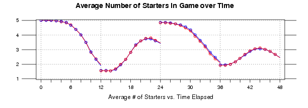
The results are summarized by the following graph:
Click Image for Full Size
First I will explain what you see in the graph above. The y-axis, from 5 to 1, is the average number of starters in the game at a given time in the game. The x-axis, from 0 to 48, is the elapsed game time. The blue dots and lines represent the home team, and the red dots and lines represent the away team.
The points represent times at which the data was captured for. The lines are drawn from smoothing splines that I fit with R for each team during each quarter.
Things to Take from This
The first thing I noticed in the data is that there does not appear to be a big difference between the substitution patterns of home versus road teams. This surprised me, but it is actually nice to know that sub patterns can’t explain much of the home court advantage. I will need to look elsewhere for that.
Also, it is interesting to notice the difference between the curves of the data from each quarter. The 1st and 3rd quarters are fairly similar in shape, but the 2nd and 4th quarters have some distinct shapes.
Reproduce These Results
In this archive you will find the data and R code I used to create the graph above and the smoothing splines fit to the data.
To run the code: extract the archive, open R, and run: source(“starters.R”)
The Next Step
Now that we’ve got a basic idea of how the average number of starters varies over time, the next step is to look at how the average number of starters changes based on the game’s point differential. After that, I will try to model how the average number of starters changes based on the game’s elapsed time and point differential.

[…] that I’ve looked at how the average number of starters changes based on time, I want to take a look at how this statistic changes based on a team’s lead (or […]